Why use polyfit and LinearRegression in the same post?

They do different jobs. numpy.polyfit returns a slope and intercept quickly so you can draw a line over a scatter plot and see whether a linear relationship is plausible before committing to anything. LinearRegression is the modelling API: it fits, predicts on new data, and plugs into the rest of scikit-learn's evaluation and pipeline tooling. Use the first to look, the second to model.

Which evaluation metric should I report?

Usually more than one, because they disagree in useful ways. Mean absolute error is in the units of your target, so "off by 2.4 on average" is a sentence anyone can act on. Mean squared error squares the errors, so it weights a few large misses much more heavily, which matters when big errors are disproportionately costly. R2 tells you the share of variance explained, which is good for comparing models but says nothing about whether the error size is acceptable for your use.

Is an R2 of 0.9888 a good result?

It is a good result on this dataset and a misleading expectation for real ones. Look at the sample rows: y tracks x almost exactly, with a small amount of noise. Nearly all the variance is explainable by construction. Real data has measurement error, omitted variables and non-linear structure, and an R2 above 0.9 on genuine business data is usually a sign of leakage rather than a great model, so it is worth checking rather than celebrating.

What do the coefficient and intercept actually tell me?

The coefficient is how much the prediction moves per one-unit change in the predictor, and the intercept is the prediction when the predictor is zero. Here a coefficient of about 1.0 and an intercept near zero mean the model learned that y is roughly equal to x, which matches what the data shows. Reading them is a cheap sanity check: a coefficient with an implausible sign or magnitude usually means a data problem rather than a modelling insight.

When does linear regression stop being the right tool?

When the relationship is not close to a straight line, when the errors grow with the size of the prediction, or when the predictors are strongly correlated with each other, which makes individual coefficients unstable and hard to interpret. Plotting residuals against predictions catches most of it: if that plot shows a curve or a fan shape rather than a formless cloud, the assumptions are not holding and a different model or a transformed target is the answer.

Journal AI Integration January 23, 2023

AI Integration · Machine Learning

Linear Regression in Python: From Data to Model

Build a linear regression model from scratch using scikit-learn, with data visualization, feature selection, and model evaluation metrics.

Anurag Verma

4 min read

Linear Regression Python Scikit-learn Machine Learning Data Science

Linear Regression in Python: From Data to Model

Key takeaways

The workflow is four steps: select predictor and target, visualise before fitting, fit with LinearRegression, then evaluate on data the model has not seen.
polyfit is for the picture and LinearRegression is for the model. Using the first to draw a line of best fit on a scatter plot is a sanity check, not a substitute for fitting properly.
Coefficients and intercept are worth reading, not just accuracy. A coefficient near 1.0 with an intercept near 0 says the model recovered the relationship almost exactly, which is a claim you can check against the data.
Report more than one metric. MAE is in the target's own units and is easy to explain; MSE punishes large errors harder; R2 says how much variance is explained. They answer different questions.
An R2 of 0.9888 here reflects a nearly noise-free dataset where y is close to x, not the accuracy you should expect on real data. Treat tutorial metrics as a check that the code works, not as a benchmark.

What is Linear Regression?

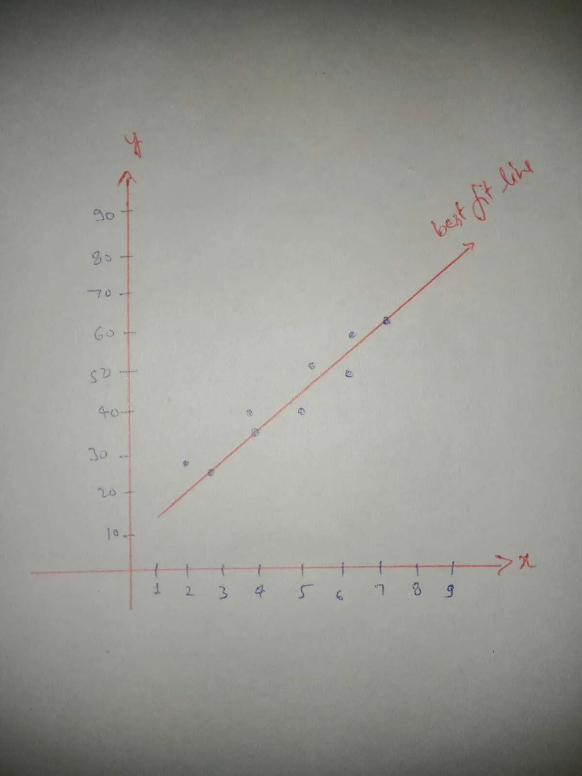
Linear regression is a statistical method used for modeling the relationship between a dependent variable (also known as the outcome or response variable) and one or more independent variables (also known as predictors or explanatory variables). The goal of linear regression is to find the best-fitting line through a set of data points, where the line is defined by an equation of the form y = mx + b, where y is the dependent variable, x is the independent variable, m is the slope of the line, and b is the y-intercept. Linear regression can be used for both simple linear regression (one independent variable) and multiple linear regression (more than one independent variable).

Linear Regression.jpeg

Importing Libraries

import pandas as pd
import numpy as np

import matplotlib.pyplot as plt
%matplotlib inline

Loding train and test dataset into pandas data frame

train_df = pd.read_csv("/kaggle/input/random-linear-regression/train.csv")
#Drop null values
train_df = train_df.dropna()
train_df.head()

	x	y
0	24.0	21.549452
1	50.0	47.464463
2	15.0	17.218656
3	38.0	36.586398
4	87.0	87.288984

test_df = pd.read_csv("/kaggle/input/random-linear-regression/test.csv")
# Drop null values
test_df = test_df.dropna()
test_df.head()

	x	y
0	77	79.775152
1	21	23.177279
2	22	25.609262
3	20	17.857388
4	36	41.849864

Selection of independent and and dependent variable

We selected the columns in your data frame that we want to use for the x and y axis. For example, if you have a column called ‘x’ that represents the independent variable and a column called ‘y’ that represents the dependent variable, you can select those columns like this:

train_x = train_df['x']
train_y = train_df['y']

test_x = test_df['x']
test_y = test_df['y']

Visualizing the training data

To draw a linear graph using your data frame, we use the popular data visualization library in Python called Matplotlib. We imported it above.

Now we use the plt.scatter() function to plot the data points, and the plt.plot() function to plot the line of best fit.

We also use the numpy.polyfit() function to fit a line to the data points and get the slope and y-intercept of the line of best fit.

coefficients = np.polyfit(train_x, train_y, 1)
m, b = coefficients
plt.scatter(train_x, train_y)
plt.plot(train_x, m*train_x + b)
plt.xlabel('train_x')
plt.ylabel('train_y')
plt.show()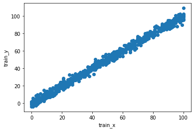

train data

Visualizing test data

coefficients = np.polyfit(test_x, test_y, 1)
m, b = coefficients
plt.scatter(test_x, test_y)
plt.plot(test_x, m*test_x + b)
plt.xlabel('test_x')
plt.ylabel('test_y')
plt.show()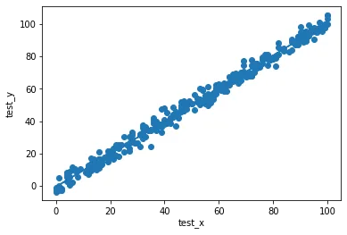

test data

Model Creation, training, and testing

To create a linear regression model and train and test the data using your data frame, we can use the scikit-learn library in Python. The first step is to import the library and the specific model you want to use.

For example, we use the LinearRegression class from the sklearn.linear_model module:

from sklearn.linear_model import LinearRegression

Create an instance of the model.

model = LinearRegression()

Now, we use the fit() method to train the model on the training data:

train_x = train_x.values.reshape(-1, 1)
test_x = test_x.values.reshape(-1, 1)

model.fit(train_x, train_y)

LinearRegression()

Check the coefficients of the model and the intercept using following command:

print("Coefficients: ",model.coef_)
print("Intercept: ",model.intercept_)

Coefficients: [1.00065638] Intercept: -0.10726546430097272

Our model is trained, now we can use the predict() method to make predictions on the test data:

y_pred = model.predict(test_x)

Evaluating model performance

We can evaluate the performance of the model by comparing the predicted values with the actual values. There are many evaluation metrics such as mean_absolute_error, mean_squared_error or r2_score.

from sklearn.metrics import mean_absolute_error, mean_squared_error, r2_score

print("Mean Absolute Error: ",mean_absolute_error(test_y, y_pred))
print("Mean Squared Error: ",mean_squared_error(test_y, y_pred))
print("R2 Score: ",r2_score(test_y, y_pred))

Mean Absolute Error: 2.415771850041258 Mean Squared Error: 9.432922192039305 R2 Score: 0.9888014444327563

Visualizing model performance

We can also visualize the results by plotting the test data points and the predicted line using the same approach as before.

plt.scatter(test_x, test_y)
plt.plot(test_x, y_pred, color='r')
plt.xlabel('x')
plt.ylabel('y')
plt.show()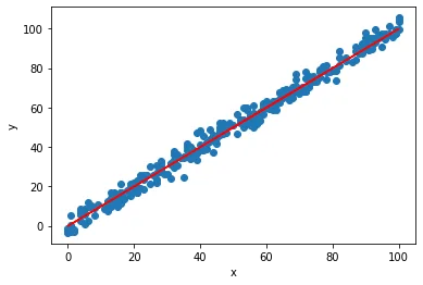

model visualization

End! Hope you like this…

GitHub link: Complete-Data-Science-Bootcamp

Main Post: Complete-Data-Science-Bootcamp

Frequently asked questions

Why use polyfit and LinearRegression in the same post?: They do different jobs. numpy.polyfit returns a slope and intercept quickly so you can draw a line over a scatter plot and see whether a linear relationship is plausible before committing to anything. LinearRegression is the modelling API: it fits, predicts on new data, and plugs into the rest of scikit-learn's evaluation and pipeline tooling. Use the first to look, the second to model.
Which evaluation metric should I report?: Usually more than one, because they disagree in useful ways. Mean absolute error is in the units of your target, so "off by 2.4 on average" is a sentence anyone can act on. Mean squared error squares the errors, so it weights a few large misses much more heavily, which matters when big errors are disproportionately costly. R2 tells you the share of variance explained, which is good for comparing models but says nothing about whether the error size is acceptable for your use.
Is an R2 of 0.9888 a good result?: It is a good result on this dataset and a misleading expectation for real ones. Look at the sample rows: y tracks x almost exactly, with a small amount of noise. Nearly all the variance is explainable by construction. Real data has measurement error, omitted variables and non-linear structure, and an R2 above 0.9 on genuine business data is usually a sign of leakage rather than a great model, so it is worth checking rather than celebrating.
What do the coefficient and intercept actually tell me?: The coefficient is how much the prediction moves per one-unit change in the predictor, and the intercept is the prediction when the predictor is zero. Here a coefficient of about 1.0 and an intercept near zero mean the model learned that y is roughly equal to x, which matches what the data shows. Reading them is a cheap sanity check: a coefficient with an implausible sign or magnitude usually means a data problem rather than a modelling insight.
When does linear regression stop being the right tool?: When the relationship is not close to a straight line, when the errors grow with the size of the prediction, or when the predictors are strongly correlated with each other, which makes individual coefficients unstable and hard to interpret. Plotting residuals against predictions catches most of it: if that plot shows a curve or a fan shape rather than a formless cloud, the assumptions are not holding and a different model or a transformed target is the answer.

Newer dispatch

Transforming Categorical Data: A Guide for Machine Learning

AI Integration

Older dispatch

Reinforcement Learning: A Comprehensive Introduction