Predicting Medical Costs with Multivariate Linear Regression

Multivariate Linear Regression

Multivariate linear regression models the relationship between multiple independent variables and a single dependent variable, extending simple linear regression beyond one predictor. It finds the equation that best predicts the dependent variable’s value from the combined effect of the independent variables, fitting coefficients that show how much each variable contributes to the prediction.

The equation is in the form of Y = a + b1X1 + b2X2 + … + bnXn, where Y is the dependent variable, X1, X2, …, Xn are the independent variables, a is the constant term, and b1, b2, …, bn are the coefficients that represent the relationship between each independent variable and the dependent variable. For a broader look at when to reach for this model versus alternatives, see our regression modeling guide.

What we do in this?

We accurately predict charges cost?

Columns present in dataset:

age: age of primary beneficiary

sex: insurance contractor gender, female, male

bmi: Body mass index, providing an understanding of body, weights that are relatively high or low relative to height, objective index of body weight (kg / m ^ 2) using the ratio of height to weight, ideally 18.5 to 24.9.

children: Number of children covered by health insurance / Number of dependents

smoker: Smoking

region: the beneficiary’s residential area in the US, northeast, southeast, southwest, northwest.

charges: Individual medical costs billed by health insurance

Importing Important libreries

import pandas as pd
import numpy as np

from sklearn.linear_model import LinearRegression
from sklearn.model_selection import train_test_split
from sklearn.metrics import mean_squared_error

import matplotlib.pyplot as plt

Reading files

Below code uses the read_csv() function from the pandas library to read in the medical insurence data from a csv file and assigns the resulting dataframe to a variable named df.

df = pd.read_csv('/kaggle/input/insurance/insurance.csv')
df.head()

	age	sex	bmi	children	smoker	region	charges
0	19	female	27.900	0	yes	southwest	16884.92400
1	18	male	33.770	1	no	southeast	1725.55230
2	28	male	33.000	3	no	southeast	4449.46200
3	33	male	22.705	0	no	northwest	21984.47061
4	32	male	28.880	0	no	northwest	3866.85520

Feature engineering

Next, we applies one-hot encoding to the sex, region, and smoker columns of the dataframe and assigns the resulting dataframe to a new variable df_encoded. Our categorical data encoding guide covers one-hot encoding and its alternatives in more depth.

# Apply one-hot encoding to "color" column
df_encoded = pd.get_dummies(df, columns=['sex', 'region', 'smoker'])
df_encoded

	age	bmi	children	charges	sex_female	sex_male	region_northeast	region_northwest	region_southeast	region_southwest	smoker_no	smoker_yes
0	19	27.900	0	16884.92400	1	0	0	0	0	1	0	1
1	18	33.770	1	1725.55230	0	1	0	0	1	0	1	0
2	28	33.000	3	4449.46200	0	1	0	0	1	0	1	0
3	33	22.705	0	21984.47061	0	1	0	1	0	0	1	0
4	32	28.880	0	3866.85520	0	1	0	1	0	0	1	0
…	…	…	…	…	…	…	…	…	…	…	…	…
1333	50	30.970	3	10600.54830	0	1	0	1	0	0	1	0
1334	18	31.920	0	2205.98080	1	0	1	0	0	0	1	0
1335	18	36.850	0	1629.83350	1	0	0	0	1	0	1	0
1336	21	25.800	0	2007.94500	1	0	0	0	0	1	1	0
1337	61	29.070	0	29141.36030	1	0	0	1	0	0	0	1

1338 rows × 12 columns

df_encoded.columns

Index([‘age’, ‘bmi’, ‘children’, ‘charges’, ‘sex_female’, ‘sex_male’, ‘region_northeast’, ‘region_northwest’, ‘region_southeast’, ‘region_southwest’, ‘smoker_no’, ‘smoker_yes’], dtype=‘object’)

Feature selection

Next, the code selects the relevant columns of the encoded dataframe to use as independent variables (X) and the dependent variable (y) for the linear regression model.

X = df_encoded[['age', 'bmi', 'children', 'sex_female', 'sex_male',
       'region_northeast', 'region_northwest', 'region_southeast',
       'region_southwest', 'smoker_no', 'smoker_yes']]
y = df_encoded['charges']

Preparing model

Below code splits the data into training and testing sets using the train_test_split function, fits the linear regression model using the training data and prints the MSE of the model. If you want a simpler single-feature version of this workflow first, our linear regression from data to model guide walks through the basics before adding multiple predictors.

# split the data into training and test sets
X_train, X_test, y_train, y_test = train_test_split(X, y, test_size=0.2)

# create a linear regression model
model = LinearRegression()

# train the model on the training data
train_loss = []
test_loss = []

# train the model
for i in range(100):
    model.fit(X_train, y_train)
    train_loss.append(mean_squared_error(y_train, model.predict(X_train)))
    test_loss.append(mean_squared_error(y_test, model.predict(X_test)))

train_score = model.score(X_train, y_train)
test_score = model.score(X_test, y_test)

# predict the values for the training and test sets
y_train_pred = model.predict(X_train)
y_test_pred = model.predict(X_test)

# Plot the prediction line
plt.scatter(y_train, y_train_pred,label='train')
plt.scatter(y_test, y_test_pred,label='test')
plt.legend()
plt.xlabel("Actual values")
plt.ylabel("Predicted values")
plt.title("Prediction line")
plt.show()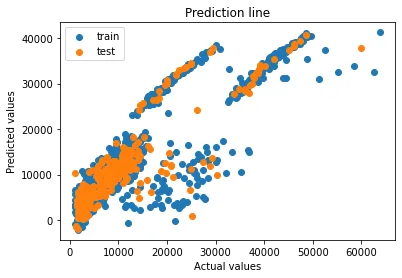

# Plot the residuals
plt.scatter(y_train_pred, y_train_pred - y_train,label='train')
plt.scatter(y_test_pred, y_test_pred - y_test,label='test')
plt.legend()
plt.xlabel("Predicted values")
plt.ylabel("Residuals")
plt.title("Residual Plot")
plt.show()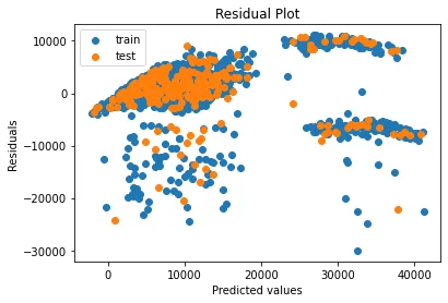

# Plot the loss
plt.plot(train_loss, label='train')
plt.plot(test_loss, label='test')
plt.legend()
plt.xlabel("Iterations")
plt.ylabel("Loss")
plt.title("Loss Plot")
plt.show()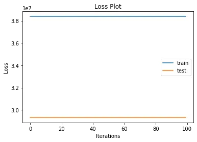

Overall, this code is performing a linear regression analysis on an insurance dataset. It begins by importing the necessary libraries for the analysis, then reads in the data from a csv file using pandas, applies one-hot encoding to certain columns, selects the relevant columns to use in the model, and finally splits the data into training and testing sets and fits a linear regression model to the training data. The last line prints the MSE of the model as a measure of performance. For more on what MSE and R² actually tell you about a model’s fit, see our evaluation metrics guide; if the gap between train and test loss grows, our overfitting and underfitting guide covers how to diagnose and fix it.

GitHub link: Complete-Data-Science-Bootcamp

Main Post: Complete-Data-Science-Bootcamp