KNN Classification: A Hands-On Guide with Python and Scikit-learn

This is a hands-on KNN classification walkthrough in Python: load a labeled dataset, scale it correctly, fit a k-nearest neighbors classifier with scikit-learn, and read the accuracy honestly instead of taking it at face value. Every step below runs as-is against the same dataset, from raw CSV to a tuned, evaluated model. If you want the theory behind why distance-based voting works before touching code, the KNN algorithm explainer covers that side.

Import necessary libraries:

A KNN classification pipeline in scikit-learn needs five libraries: numpy and pandas for loading and reshaping data, seaborn and matplotlib for visualizing class separation before modeling, and scikit-learn itself for the KNeighborsClassifier, the train/test split, feature scaling, and accuracy scoring used later in this walkthrough.

import numpy as np
import pandas as pd
import seaborn as sns
import matplotlib.pyplot as plt
from sklearn.neighbors import KNeighborsClassifier
from sklearn.model_selection import train_test_split
from sklearn.preprocessing import StandardScaler
from sklearn.metrics import accuracy_score

Load the data:

The code reads a csv file containing the dataset into a pandas dataframe using pd.read_csv() method.

# Load your data into a pandas dataframe
df = pd.read_csv("/kaggle/input/knn-data1/KNN_Project_Data")

df

	XVPM	GWYH	TRAT	TLLZ	IGGA	HYKR	EDFS	GUUB	MGJM	JHZC	TARGET CLASS
0	1636.670614	817.988525	2565.995189	358.347163	550.417491	1618.870897	2147.641254	330.727893	1494.878631	845.136088	0
1	1013.402760	577.587332	2644.141273	280.428203	1161.873391	2084.107872	853.404981	447.157619	1193.032521	861.081809	1
2	1300.035501	820.518697	2025.854469	525.562292	922.206261	2552.355407	818.676686	845.491492	1968.367513	1647.186291	1
3	1059.347542	1066.866418	612.000041	480.827789	419.467495	685.666983	852.867810	341.664784	1154.391368	1450.935357	0
4	1018.340526	1313.679056	950.622661	724.742174	843.065903	1370.554164	905.469453	658.118202	539.459350	1899.850792	0
…	…	…	…	…	…	…	…	…	…	…	…
995	1343.060600	1289.142057	407.307449	567.564764	1000.953905	919.602401	485.269059	668.007397	1124.772996	2127.628290	0
996	938.847057	1142.884331	2096.064295	483.242220	522.755771	1703.169782	2007.548635	533.514816	379.264597	567.200545	1
997	921.994822	607.996901	2065.482529	497.107790	457.430427	1577.506205	1659.197738	186.854577	978.340107	1943.304912	1
998	1157.069348	602.749160	1548.809995	646.809528	1335.737820	1455.504390	2788.366441	552.388107	1264.818079	1331.879020	1
999	1287.150025	1303.600085	2247.287535	664.362479	1132.682562	991.774941	2007.676371	251.916948	846.167511	952.895751	1

1000 rows × 11 columns

Data visualization:

The code creates a scatter plot matrix using the sns.pairplot method from the seaborn library and plots it using the plt.show method from the matplotlib library. This scatter plot matrix is used to visualize the relationships between the variables in the data.

# scatter plot matrix
sns.pairplot(df, hue='TARGET CLASS')
plt.show()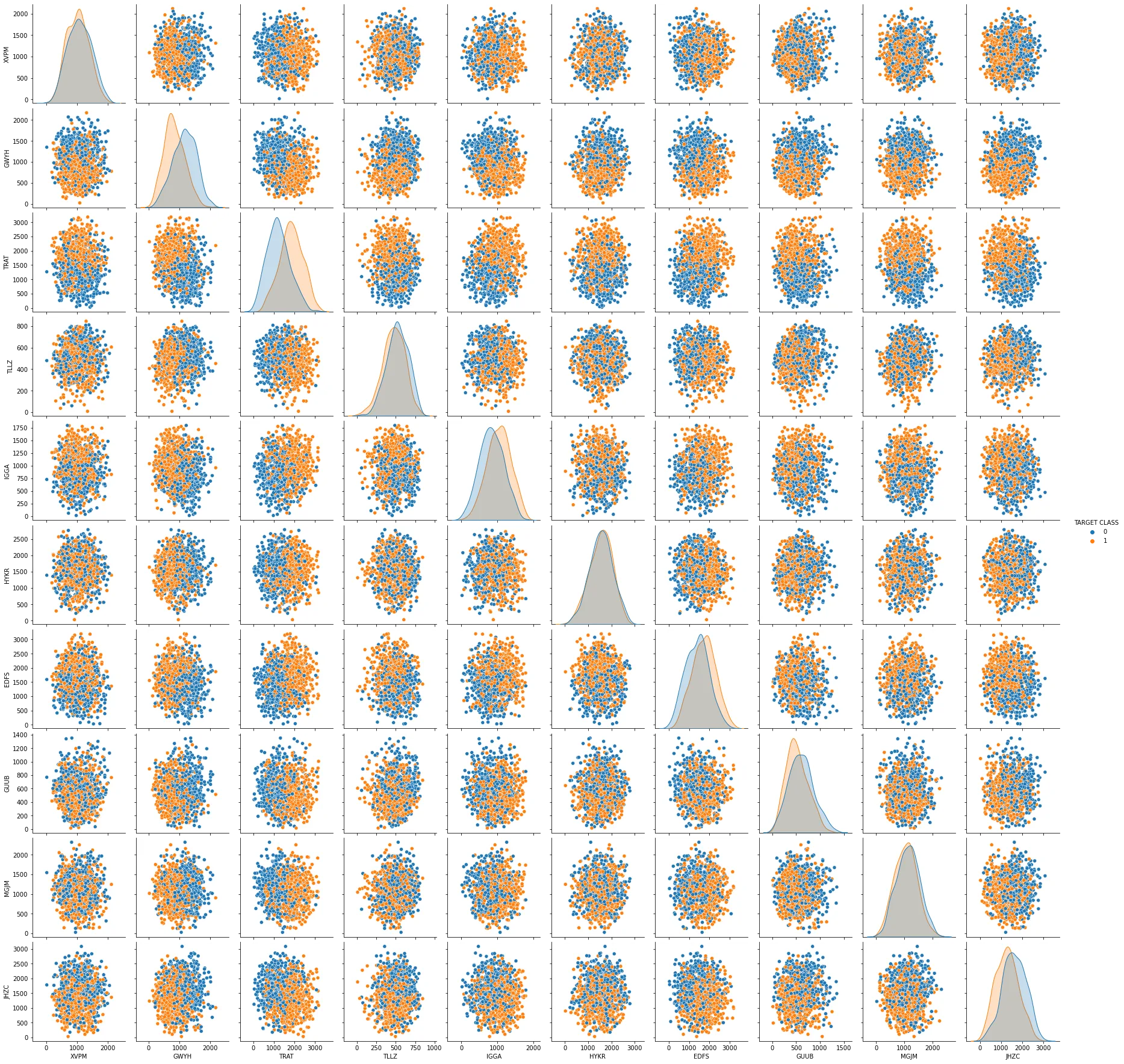

Split the dataset into training and testing sets:

The code splits the dataset into two parts: training and testing. The train_test_split method from scikit-learn is used to split the data into 80% training data and 20% testing data. The X variable is assigned the values of the dataframe with the target column dropped and y variable is assigned the values of the target column.

# Split the dataset into training and testing sets
X = df.drop("TARGET CLASS", axis=1)
y = df["TARGET CLASS"]
X_train, X_test, y_train, y_test = train_test_split(X, y, test_size=0.2, random_state=42)

Pre-process the data:

The code scales the data using the StandardScaler method from scikit-learn. The method fit_transform is applied to the training data and transform is applied to the testing data. This scaling is necessary because different features in the data have different ranges, and it is important to pre-process the data before applying a machine learning model.

# Pre-process the data
scaler = StandardScaler()
X_train = scaler.fit_transform(X_train)
X_test = scaler.transform(X_test)

Training and testing the KNN model:

The code trains a K-nearest neighbors (KNN) model using the training data and the KNeighborsClassifier method from scikit-learn. The KNN model is then tested using the testing data, and the accuracy of the model is calculated using the accuracy_score method from scikit-learn.

# Train the KNN model
knn = KNeighborsClassifier(n_neighbors=5)
knn.fit(X_train, y_train)

KNeighborsClassifier()

# Evaluate the model
y_pred = knn.predict(X_test)
accuracy = accuracy_score(y_test, y_pred)
print("Accuracy:", accuracy*100)

Accuracy: 82.0

Choosing k instead of accepting the default:

n_neighbors=5 is scikit-learn’s default, not a value tuned for this dataset. The standard way to pick k is an error-rate sweep: fit the model at several odd values of k, record the validation error at each, and look for the point where error stops dropping.

# Sweep k and record the error rate at each value
error_rates = []

for k in range(1, 40, 2):
    knn_k = KNeighborsClassifier(n_neighbors=k)
    knn_k.fit(X_train, y_train)
    pred_k = knn_k.predict(X_test)
    error_rates.append(np.mean(pred_k != y_test))

plt.plot(range(1, 40, 2), error_rates, marker='o')
plt.xlabel('k')
plt.ylabel('Error rate')
plt.show()

Odd values avoid ties in a two-class vote. The plot typically shows a steep drop, a flat basin, and then a slow climb as k grows large enough to average across the actual class boundary, the same underfitting-versus-overfitting tradeoff covered in bias vs. variance in predictive modeling. Pick k from inside that basin, not from whichever value happens to look lowest by a single point, since that can just be noise in this particular train/test split. Manually sweeping k works fine for one hyperparameter; once you’re tuning several at once, GridSearchCV does the same search more systematically.

Reading the results beyond accuracy:

Accuracy alone hides how the errors are distributed. A confusion matrix and a classification report show whether the model is making one type of mistake more than another, which matters more once the two classes are not perfectly balanced.

from sklearn.metrics import confusion_matrix, classification_report

print(confusion_matrix(y_test, y_pred))
print(classification_report(y_test, y_pred))

The confusion matrix breaks the 82% down into true positives, true negatives, false positives, and false negatives. The classification report adds precision and recall per class, which is the number to check before trusting accuracy on any dataset where one class shows up more often than the other, the full set of tradeoffs is covered in classification and regression evaluation metrics. On this dataset the classes are close to balanced, which is part of why a single accuracy number is a reasonable summary here, that would not hold on a fraud- or churn-style dataset where the minority class is the one that matters.

This notebook is one piece of a longer sequence; the 100-day data science roadmap has the full path from Python basics through model evaluation if you want the surrounding context.

GitHub link: Complete-Data-Science-Bootcamp

Main Post: Complete-Data-Science-Bootcamp