Support Vector Machines (SVM): Theory and Hands-On Classification

Support Vector Machines (SVM) is a widely used Supervised Learning algorithm that is used for both Classification and Regression tasks in Machine Learning. Although it is primarily employed for Classification problems. It sits alongside other classic classifiers like K-Nearest Neighbors and decision trees as a standard tool to reach for on a labeled dataset.

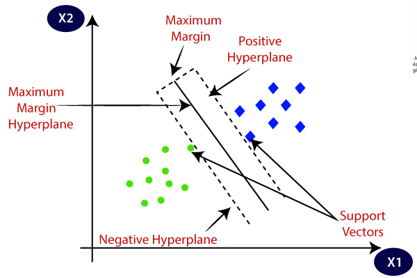
The objective of the SVM algorithm is to find the best line, known as the hyperplane, which can effectively divide n-dimensional space into different classes. This makes it possible to accurately place new data points into the appropriate category.

To determine the hyperplane, SVM selects the extreme cases, known as support vectors, that contribute to its creation. The algorithm is named as Support Vector Machine due to these support vectors. The following illustration shows two distinct categories being classified by a hyperplane or decision boundary:

Types of SVM

Support Vector Machines come in two types, split by whether the data can be separated with a straight line. Linear SVM handles data where a single straight line (or a flat hyperplane in higher dimensions) cleanly divides the classes. Non-Linear SVM handles data that no straight line can separate, using the kernel trick to map it into a higher-dimensional space where a linear split becomes possible.

There are two types of Support Vector Machines (SVM):

Linear SVM: This type of SVM is employed for linearly separable data. In other words, if a dataset can be divided into two classes using a single straight line, it is considered linearly separable, and a Linear SVM classifier is used for this purpose.

Non-Linear SVM: Non-Linear SVM is used for datasets that cannot be classified using a straight line. In such cases, this type of SVM is applied to separate the non-linearly separated data.

Working of Linear SVM

Linear SVM is a type of SVM that is used for linearly separable data. It works by creating the best line or hyperplane that separates the two classes in a two-dimensional plane.

Consider a simple example of a two-class classification problem, where we have two classes of points in a two-dimensional plane as shown below:

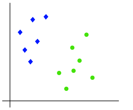
Here, we want to separate the blue and red points into two different classes using a line. The objective of Linear SVM is to find the line that separates these classes with the maximum margin. The margin is the distance between the line and the closest data points from both classes. The best line is the one that has the maximum margin, which is also known as the maximum margin classifier.

In this example, the line that separates the blue and red points with the maximum margin is the line drawn in green. The points closest to the line are called support vectors, and they play a key role in defining the best line. In the above example, the support vectors are the points closest to the line, as shown by the dotted lines.

The line that separates the two classes with the maximum margin is the best line, and this is what Linear SVM aims to find. The hyperplane is then used to classify new data points into either class, depending on which side of the line the new data point lies.

Working of Non-Linear SVM

Non-Linear SVM is a type of SVM used for non-linearly separable data. In such cases, the algorithm transforms the input data into a higher-dimensional space, where a linear separation becomes possible.

For example, consider a two-class classification problem where the data points are not linearly separable in a two-dimensional plane, as shown below:

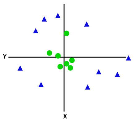
Here, it is not possible to separate the blue and red points into two different classes using a straight line. To overcome this, Non-Linear SVM uses a technique called kernel trick, where it maps the input data into a higher-dimensional space, where the data points become linearly separable.

In the above example, the data points are transformed into a three-dimensional space using a radial basis function (RBF) kernel. In the higher-dimensional space, a linear separation is now possible, as shown below:

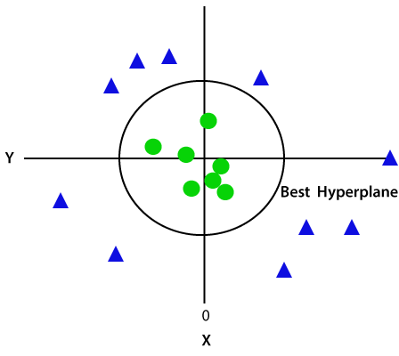
Here, the red and blue points are separated by a hyperplane, and this hyperplane is used to classify new data points. The mapping from the input data to the higher-dimensional space is done implicitly by the Non-Linear SVM algorithm, and the user does not need to be aware of the mapping.

Non-Linear SVM works by transforming the input data into a higher-dimensional space where a linear separation becomes possible, and a hyperplane is used to separate the data points into different classes.

Python implementation of Linear SVM

import numpy as np
import matplotlib.pyplot as plt
from sklearn import datasets
from sklearn.svm import SVC

# Load the iris dataset
iris = datasets.load_iris()
X = iris["data"][:, (2, 3)]  # petal length, petal width
y = iris["target"]

# Train a linear SVM
svm_clf = SVC(kernel="linear", C=float("inf"))
svm_clf.fit(X, y)

# Visualize the data and the decision boundary
plt.scatter(X[:, 0], X[:, 1], c=y, s=30, cmap=plt.cm.Paired)
plt.show()

# Get the separating hyperplane
w = svm_clf.coef_[0]
b = svm_clf.intercept_[0]
x_min, x_max = X[:, 0].min() - 1, X[:, 0].max() + 1
y_min, y_max = X[:, 1].min() - 1, X[:, 1].max() + 1
xx, yy = np.meshgrid(np.arange(x_min, x_max, 0.2), np.arange(y_min, y_max, 0.2))
Z = svm_clf.predict(np.c_[xx.ravel(), yy.ravel()])
Z = Z.reshape(xx.shape)
plt.contourf(xx, yy, Z, cmap=plt.cm.Paired, alpha=0.8)
plt.xlim(xx.min(), xx.max())
plt.ylim(yy.min(), yy.max())

plt.show()

In the code above, we first load the iris dataset and extract the petal length and width as the feature variables. We then train a linear SVM using the SVC class from the scikit-learn library, with kernel=“linear” and C=float(“inf”) to enforce a hard margin. If you haven’t tuned an SVM’s hyperparameters before, our GridSearchCV guide to scikit-learn hyperparameter tuning covers searching over C and kernel choice systematically instead of by hand.

Next, we visualize the data and the decision boundary by plotting the data points and the contours of the decision boundary. The decision boundary is obtained by calling the predict method on a grid of points in the feature space, and reshaping the output to form a 2D image. The final plot shows the decision boundary and the data points, with the different colors indicating the different classes in the target variable.

Python implementation of Non-Linear SVM

import numpy as np
import matplotlib.pyplot as plt
from sklearn import datasets
from sklearn.svm import SVC

# Load the moons dataset
moons = datasets.make_moons(n_samples=100, noise=0.15)
X = moons[0]
y = moons[1]

# Train a non-linear SVM
svm_clf = SVC(kernel="rbf", gamma=5, C=0.001)
svm_clf.fit(X, y)

SVC(C=0.001, gamma=5)

# Visualize the data and the decision boundary
plt.scatter(X[:, 0], X[:, 1], c=y, s=30, cmap=plt.cm.Paired)
plt.show()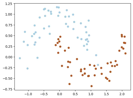

# Get the separating hyperplane
x_min, x_max = X[:, 0].min() - 1, X[:, 0].max() + 1
y_min, y_max = X[:, 1].min() - 1, X[:, 1].max() + 1
xx, yy = np.meshgrid(np.arange(x_min, x_max, 0.2), np.arange(y_min, y_max, 0.2))
Z = svm_clf.predict(np.c_[xx.ravel(), yy.ravel()])
Z = Z.reshape(xx.shape)
plt.contourf(xx, yy, Z, cmap=plt.cm.Paired, alpha=0.8)
plt.xlim(xx.min(), xx.max())
plt.ylim(yy.min(), yy.max())

plt.show()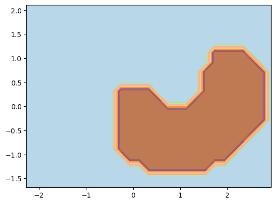

In the code above, we first generate a non-linear dataset using the make_moons function from the scikit-learn library. We then train a non-linear SVM using the SVC class from the scikit-learn library, with kernel=“rbf” (Radial basis function) and gamma=5 and C=0.001 to control the complexity of the model.

Next, we visualize the data and the decision boundary by plotting the data points and the contours of the decision boundary. The decision boundary is obtained by calling the predict method on a grid of points in the feature space, and reshaping the output to form a 2D image. The final plot shows the decision boundary and the data points, with the different colors indicating the different classes in the target variable.

Once you have a fitted SVM, judge it the same way you’d judge any classifier: with a confusion matrix and per-class precision and recall rather than accuracy alone, covered in our classification and regression evaluation metrics guide. If you want to see the same kind of scikit-learn workflow applied with a different algorithm, our Naive Bayes sentiment analysis walkthrough builds a comparable pipeline end to end.

GitHub link: Complete-Data-Science-Bootcamp

Main Post: Complete-Data-Science-Bootcamp