RAG Architecture in 2026: From Vector Search to Production

Retrieval-Augmented Generation has matured far beyond “embed your documents, find the nearest neighbors, stuff them into a prompt.” The naive vector search pipeline that dominated 2023 and 2024 now sits at the bottom of a growing stack of retrieval techniques, sparse retrieval, sparse attention over long context, and hybrid search among them, each solving different failure modes that production teams encounter at scale.

We spent the past several months evaluating retrieval architectures across three production systems: a legal document QA platform, a developer documentation assistant, and a multi-tenant customer support bot. This post documents what we found: what works, what fails, and where each approach sits on the complexity-performance tradeoff curve. If you’re building the agent layer that sits on top of this retrieval stack, our guide to production Model Context Protocol deployments covers the piece we don’t get into here.

The Problem with Naive Vector Search

The original RAG pipeline was elegant in its simplicity. Chunk your documents, embed each chunk with a model like text-embedding-ada-002, store vectors in a database, retrieve the top-k nearest neighbors at query time, and concatenate them into the LLM context window.

This approach has three systemic failure modes that become unavoidable at scale:

1. Semantic drift. Embedding models compress meaning into fixed-dimension vectors. Queries that hinge on exact terminology (legal clauses, API parameter names, medical codes) get mapped to neighborhoods of semantically similar but factually wrong chunks.
2. Chunking artifacts. Splitting documents at arbitrary token boundaries destroys context. A chunk containing “the exception to this rule is…” means nothing without the preceding chunk that defines the rule.
3. Query-document mismatch. User queries and document passages occupy different linguistic registers. “How do I fix the timeout error?” and “Connection timeout occurs when the socket pool is exhausted” are semantically related but sit far apart in embedding space.

In our legal QA benchmark, naive dense retrieval returned the correct chunk in the top-5 results only 62% of the time. After switching to a hybrid pipeline, that number climbed to 89%.

The 2026 Retrieval Landscape

The retrieval layer is no longer a single technique. It is an ensemble. Here is where the major approaches stand.

Approach	Retrieval Quality	Latency (p95)	Index Size Overhead	Implementation Complexity
Dense bi-encoder (e.g., OpenAI embeddings)	Moderate	~15ms	1x (baseline)	Low
Sparse retrieval (BM25)	Good for exact match	~5ms	0.3x	Low
SPLADE v3	High	~20ms	0.8x	Medium
ColBERT v2.5	Very High	~35ms	3-5x	High
Hybrid (dense + sparse + reranker)	Very High	~60ms	1.5x	Medium-High
Contextual retrieval (Anthropic-style)	Highest	~80ms	1.2x	High

Let us walk through each.

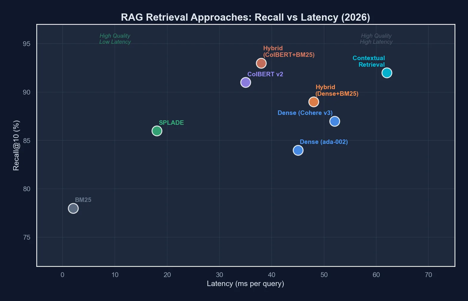A modern RAG pipeline routes queries through multiple retrieval paths and merges results via a learned reranker before generation.

Dense Retrieval: The Baseline

Dense bi-encoder retrieval remains the starting point. Models like OpenAI’s text-embedding-3-large, Cohere’s embed-v4, and open-source alternatives like bge-m3 project both queries and documents into a shared embedding space.

The core operation is straightforward:

from openai import OpenAI
import numpy as np

client = OpenAI()

def embed(texts: list[str], model: str = "text-embedding-3-large") -> np.ndarray:
    response = client.embeddings.create(input=texts, model=model)
    return np.array([e.embedding for e in response.data])

query_vec = embed(["How do I configure retry logic?"])
doc_vecs = embed(chunks)  # pre-computed and stored

# Cosine similarity retrieval
similarities = np.dot(doc_vecs, query_vec.T).flatten()
top_k_indices = np.argsort(similarities)[-10:][::-1]

Dense retrieval excels at capturing broad semantic similarity. It handles paraphrasing well and generalizes across vocabulary. But it compresses all meaning into a single vector, which inevitably loses fine-grained token-level information.

Sparse Retrieval: BM25 Is Not Dead

BM25, the algorithm that powered search engines for decades, remains remarkably competitive. It matches on exact terms, handles rare vocabulary well, and requires no GPU inference at query time.

In our developer documentation benchmark, BM25 outperformed dense retrieval on queries containing specific function names, error codes, and configuration parameters: precisely the queries where exact lexical matching matters most.

from rank_bm25 import BM25Okapi

tokenized_corpus = [doc.split() for doc in chunks]
bm25 = BM25Okapi(tokenized_corpus)

query = "ConnectionPoolTimeout retry backoff"
scores = bm25.get_scores(query.split())
top_k = np.argsort(scores)[-10:][::-1]

The weakness is obvious: BM25 cannot handle synonyms, paraphrasing, or conceptual similarity. “Authentication failure” and “login error” are invisible to each other.

SPLADE: Learned Sparse Representations

SPLADE (SParse Lexical AnD Expansion) occupies a fascinating middle ground. It uses a transformer to produce sparse, high-dimensional vectors where each dimension corresponds to a vocabulary token. The model learns to activate relevant tokens, including tokens that do not appear in the original text, creating an expanded sparse representation.

from transformers import AutoModelForMaskedLM, AutoTokenizer
import torch

model_name = "naver/splade-v3"
tokenizer = AutoTokenizer.from_pretrained(model_name)
model = AutoModelForMaskedLM.from_pretrained(model_name)

def splade_encode(text: str) -> dict[str, float]:
    tokens = tokenizer(text, return_tensors="pt", truncation=True)
    with torch.no_grad():
        logits = model(**tokens).logits
    # Max pooling over sequence length, then ReLU + log
    weights = torch.max(
        torch.log1p(torch.relu(logits)) * tokens["attention_mask"].unsqueeze(-1),
        dim=1
    ).values.squeeze()
    # Extract non-zero dimensions
    indices = weights.nonzero().squeeze()
    values = weights[indices]
    vocab = tokenizer.get_vocab()
    inv_vocab = {v: k for k, v in vocab.items()}
    return {inv_vocab[idx.item()]: val.item() for idx, val in zip(indices, values)}

SPLADE’s learned expansion means that a document about “authentication” will activate the “login” token even if the word never appears. This gives it the interpretability and efficiency of sparse retrieval with some of the generalization capacity of dense models.

SPLADE vectors can be stored in any inverted index (Elasticsearch, Lucene, Vespa), making adoption straightforward for teams already running a search stack. No separate vector database required.

ColBERT: Late Interaction Changes Everything

ColBERT (Contextualized Late Interaction over BERT) takes a fundamentally different approach. Instead of compressing each document into a single vector, ColBERT retains per-token embeddings for both queries and documents. Relevance is computed via a “late interaction” mechanism: a MaxSim operation that finds the best-matching document token for each query token.

# Pseudocode for ColBERT MaxSim scoring
def colbert_score(query_embeddings, doc_embeddings):
    """
    query_embeddings: (num_query_tokens, dim)
    doc_embeddings: (num_doc_tokens, dim)
    """
    # For each query token, find max similarity across all doc tokens
    similarity_matrix = query_embeddings @ doc_embeddings.T  # (Q, D)
    max_similarities = similarity_matrix.max(dim=1).values   # (Q,)
    return max_similarities.sum()

This per-token interaction preserves granular matching information that single-vector approaches discard. ColBERT can distinguish between “Python list comprehension” and “Python list methods” because it retains the individual token representations.

The tradeoff is storage. Each document requires storing all of its token embeddings, which typically means 3-5x the index size compared to single-vector dense retrieval. ColBERT v2 and its successors introduced residual compression to mitigate this, but it remains the most storage-intensive approach.

Method	Tokens Stored per Document	Dims per Token	Bytes per 1K Documents (avg 200 tokens)
Dense bi-encoder	1	1536	~6 MB
ColBERT v2 (compressed)	~200	128	~25 MB
ColBERT v2.5 (quantized)	~200	128 (2-bit)	~8 MB
SPLADE v3	~100 (sparse)	1 (weight)	~1 MB

Hybrid Search: The Production Default

In every production system we evaluated, the best results came from combining multiple retrieval signals. The pattern that emerged as the default architecture in 2026 follows a two-stage pipeline:

Stage 1, Parallel retrieval across multiple indices:

• Dense vector search (semantic similarity)
• Sparse BM25 or SPLADE (lexical precision)
• Optionally, ColBERT late interaction (token-level matching)

Stage 2, Cross-encoder reranking to merge and re-score the combined candidate set.

from typing import NamedTuple

class RetrievalResult(NamedTuple):
    chunk_id: str
    score: float
    source: str

def hybrid_retrieve(
    query: str,
    dense_index,
    sparse_index,
    reranker,
    top_k: int = 10,
    candidates_per_source: int = 30,
) -> list[RetrievalResult]:
    # Stage 1: parallel retrieval
    dense_results = dense_index.search(query, k=candidates_per_source)
    sparse_results = sparse_index.search(query, k=candidates_per_source)

    # Deduplicate by chunk_id
    candidate_ids = set()
    candidates = []
    for result in dense_results + sparse_results:
        if result.chunk_id not in candidate_ids:
            candidate_ids.add(result.chunk_id)
            candidates.append(result)

    # Stage 2: cross-encoder reranking
    reranked = reranker.rerank(
        query=query,
        documents=[get_chunk_text(c.chunk_id) for c in candidates],
        top_k=top_k,
    )

    return reranked

The cross-encoder reranker is the critical component. Unlike bi-encoders that process queries and documents independently, cross-encoders process the query-document pair together through a full transformer, enabling deep token-level interactions. Models like Cohere Rerank v3, bge-reranker-v2.5-gemma2, and Jina Reranker v2 have made this step both accurate and fast enough for production.

Cross-encoder reranking adds 30-50ms of latency per query. In latency-sensitive applications, consider limiting the candidate pool to 30-50 documents and running the reranker on GPU. CPU inference on larger candidate sets can push p95 latency above 200ms.

Contextual Retrieval: Prepending Context Before Embedding

Anthropic introduced contextual retrieval as a technique to solve the chunking artifact problem. The idea is deceptively simple: before embedding each chunk, prepend a short context paragraph that explains where the chunk sits within its source document. The examples below use Claude Haiku for this step; see our rundown of Claude Opus 4.6’s context handling if you’re deciding which model tier fits which stage of your pipeline.

import anthropic

client = anthropic.Anthropic()

def generate_chunk_context(
    document: str,
    chunk: str,
) -> str:
    response = client.messages.create(
        model="claude-sonnet-4-20250514",
        max_tokens=200,
        messages=[{
            "role": "user",
            "content": f"""<document>
{document}
</document>

Here is the chunk we want to situate within the document:
<chunk>
{chunk}
</chunk>

Give a short (2-3 sentence) context that explains what this chunk
covers and how it relates to the rest of the document. Respond with
only the context, nothing else."""
        }],
    )
    return response.content[0].text

def create_contextual_chunk(document: str, chunk: str) -> str:
    context = generate_chunk_context(document, chunk)
    return f"{context}\n\n{chunk}"

This contextualized chunk is then embedded and indexed normally. At query time, the retrieval process is unchanged. The context is already baked into the embedding.

The results we observed were significant. On our legal QA benchmark, contextual retrieval improved recall@10 by 14 percentage points over standard chunking with the same embedding model. The technique is model-agnostic and composable with every other approach in this post.

The cost is incurred at indexing time: every chunk requires an LLM call to generate its context. For a corpus of 100,000 chunks, that is 100,000 API calls. Using a cost-efficient model like Claude Haiku or GPT-4o mini makes this feasible, but it is a non-trivial cost that must be factored into the pipeline.

Production RAG Architecture

Putting it all together, a production RAG pipeline in 2026 looks like this:

# rag-pipeline-config.yaml
ingestion:
  chunking:
    strategy: "recursive_character"
    chunk_size: 512
    overlap: 64
    separators: ["\n## ", "\n### ", "\n\n", "\n", ". "]
  contextual_retrieval:
    enabled: true
    model: "claude-haiku-4-20250514"
    max_context_tokens: 150
  embedding:
    models:
      - name: "dense"
        model_id: "text-embedding-3-large"
        dimensions: 1536
      - name: "sparse"
        model_id: "splade-v3"
        type: "learned_sparse"
  indexing:
    dense_store: "pgvector"  # or qdrant, pinecone, weaviate
    sparse_store: "elasticsearch"
    sync: "on_commit"

retrieval:
  stage_1:
    dense:
      top_k: 40
      similarity: "cosine"
    sparse:
      top_k: 40
      algorithm: "splade_v3"
    fusion:
      method: "reciprocal_rank_fusion"
      k_constant: 60
  stage_2:
    reranker:
      model: "cohere-rerank-v3.5"
      top_k: 10
  stage_3:
    generation:
      model: "claude-sonnet-4-20250514"
      max_context_chunks: 8
      system_prompt_template: "answer_with_citations"

evaluation:
  framework: "ragas"
  metrics:
    - "faithfulness"
    - "answer_relevancy"
    - "context_precision"
    - "context_recall"
  schedule: "weekly"

Continuous evaluation with RAGAS metrics creates a feedback loop that identifies retrieval degradation before it affects users.

Reciprocal Rank Fusion

When merging results from multiple retrieval sources, Reciprocal Rank Fusion (RRF) provides a parameter-free method that avoids the need to normalize scores across different systems:

def reciprocal_rank_fusion(
    result_lists: list[list[str]],
    k: int = 60,
) -> list[tuple[str, float]]:
    """
    Merge ranked lists using RRF.
    k is a constant that controls the impact of high-ranking documents.
    """
    scores: dict[str, float] = {}
    for result_list in result_lists:
        for rank, doc_id in enumerate(result_list):
            scores[doc_id] = scores.get(doc_id, 0) + 1.0 / (k + rank + 1)

    sorted_results = sorted(scores.items(), key=lambda x: x[1], reverse=True)
    return sorted_results

RRF works well because it is rank-based rather than score-based. Dense cosine similarities, BM25 scores, and SPLADE weights all exist on different scales. Normalizing them requires careful calibration. RRF sidesteps this entirely.

Evaluation with RAGAS

You cannot improve what you do not measure. RAGAS (Retrieval Augmented Generation Assessment) has become the standard evaluation framework for RAG pipelines. It provides four core metrics:

Metric	What It Measures	How It Works
Faithfulness	Are generated answers grounded in retrieved context?	LLM decomposes the answer into claims, then checks each against context
Answer Relevancy	Does the answer address the question?	Generates hypothetical questions from the answer, measures similarity to original
Context Precision	Are relevant chunks ranked higher than irrelevant ones?	Checks if ground-truth-relevant chunks appear early in the retrieval list
Context Recall	Are all necessary chunks retrieved?	Compares retrieved context against ground truth answers

from ragas import evaluate
from ragas.metrics import (
    faithfulness,
    answer_relevancy,
    context_precision,
    context_recall,
)
from datasets import Dataset

eval_dataset = Dataset.from_dict({
    "question": questions,
    "answer": generated_answers,
    "contexts": retrieved_contexts,  # list of list of strings
    "ground_truth": ground_truth_answers,
})

results = evaluate(
    dataset=eval_dataset,
    metrics=[
        faithfulness,
        answer_relevancy,
        context_precision,
        context_recall,
    ],
)

print(results)
# {'faithfulness': 0.89, 'answer_relevancy': 0.92,
#  'context_precision': 0.85, 'context_recall': 0.78}

We run RAGAS evaluations on a curated test set of 200 question-answer pairs every week. This caught a regression when we updated our embedding model. Context recall dropped 8 points because the new model handled technical abbreviations differently. Without automated evaluation, that regression would have reached production.

When RAG Beats Fine-Tuning

The RAG versus fine-tuning decision comes up in every AI engineering project. After building both approaches across multiple domains, here is our decision framework.

Choose RAG when:

• Your knowledge base changes frequently (weekly or more)
• You need verifiable citations and source attribution
• You require multi-tenant data isolation
• Your corpus exceeds what fits in a fine-tuning dataset
• Accuracy on factual recall matters more than stylistic consistency

Choose fine-tuning when:

• You need the model to adopt a specific tone, format, or reasoning style
• The knowledge is relatively static
• Latency is critical and you cannot afford retrieval overhead
• You want to encode domain-specific reasoning patterns, not just facts

Use both when:

• You fine-tune for style and reasoning, then augment with RAG for current facts
• The fine-tuned model handles the “how to answer” while RAG handles the “what to answer with”

In our customer support system, a fine-tuned model alone achieved 71% answer accuracy. RAG alone reached 83%. A fine-tuned model with RAG hit 91%. The fine-tuning taught the model the company's communication style and escalation logic, while RAG provided the current policy documents and product specifications.

Sparse Attention and Long-Context Alternatives

An emerging alternative to retrieval is simply using longer context windows. Models like Gemini 2.0 Pro with its 2M token context and Claude with 200K tokens can ingest entire document corpora without chunking.

However, our benchmarks tell a more complicated story. We tested “long-context stuffing” against RAG on a 500-document corpus:

• Long-context (all documents in prompt): 85% answer accuracy, $0.42 per query, 8.2s latency
• RAG (top-8 chunks): 89% answer accuracy, $0.03 per query, 1.4s latency

Long context is simpler to implement but becomes cost-prohibitive at scale. For production systems handling thousands of queries per day, RAG remains the economical choice.

Sparse attention mechanisms used internally by models like Mistral, Jamba, and DeepSeek-V3 (which we cover in more detail in our DeepSeek and Qwen open-source surge writeup) reduce the quadratic cost of self-attention. These architectures make long contexts computationally feasible, but the per-token cost of input processing still makes RAG more cost-efficient for most production workloads. Smaller, domain-specific models are also changing this calculus; see our piece on small language models in production for where a narrower model plus RAG beats a frontier model with a huge context window.

Practical Recommendations

After evaluating these approaches across three production systems and months of iteration, here is our distilled guidance:

1. Start with hybrid search. Dense embeddings plus BM25 with reciprocal rank fusion gives 80% of the quality improvement for 20% of the complexity. Add a cross-encoder reranker when quality requirements tighten.

2. Invest in chunking strategy. Recursive character splitting with semantic boundaries (headers, paragraphs) outperforms naive fixed-size chunking by 10-15 percentage points on recall. Consider contextual retrieval if your corpus has interconnected sections.

3. Measure from day one. Set up RAGAS or an equivalent evaluation framework before optimizing retrieval. Without metrics, you are tuning parameters in the dark.

4. ColBERT is worth it for high-stakes domains. Legal, medical, and financial applications where retrieval errors have real consequences justify ColBERT’s storage and complexity costs. For general-purpose chatbots and documentation search, hybrid dense+sparse is sufficient.

5. Do not ignore the generation prompt. Retrieval quality is necessary but not sufficient. A well-structured system prompt that instructs the LLM to cite sources, acknowledge uncertainty, and stay grounded in context prevents hallucination as much as better retrieval does.

6. Plan for evaluation drift. Your test set will become stale as your corpus evolves. Budget time to update evaluation data quarterly. Stale benchmarks give false confidence.

If your retrieval pipeline hands off to a multi-step agent rather than a single generation call, the orchestration layer needs the same evaluation discipline; our agentic workflow orchestration guide covers that side of the system.

The RAG ecosystem in 2026 offers a rich toolkit of retrieval techniques, each with distinct strengths. The engineering challenge is no longer finding the single best approach. It is composing the right combination for your specific constraints on accuracy, latency, cost, and operational complexity.